Next: 3 Introduction to Data Flow Graph Design Up: Appnotes Index Previous:1 Executive Summary
![]()
![]()
![]()
![]()
Next: 3 Introduction to Data Flow Graph Design
Up: Appnotes Index
Previous:1 Executive Summary
These are design options that must be explored as part of the design process in order to be able to generate efficient and compact code for the target DSPs. While it may be desirable to be able to perform these processes automatically, the tools that automate these tasks have not yet been developed to a mature state so they can be used routinely used. The mature tools, like GEDAE™, that are availabel now assist the intelligent designer to be more productive in considering more design options.
The basic graphical tool used to develop the Data Flow design is the Data Flow graph. In order to understand how this graphical concept captures the complete functionality of the signal processing algorithm, we must first re-examine the basic method of expressing a mathematical description of a signal processing algorithm by a graphical description. The resultant graphical description provides the insight into the structure of the equations and aids the parallelization of the algorithm. This section provides a description of a computational graph and then shows what is required to convert this to a Data Flow Graph.
The functional representation incorporates both binary and unitary operators. For example, if we have c = a + b we can change this representation to be c = add(a,b) or using the symbol + for the function add, we have c = +(a,b). In the case of the unitary operation we have c = -a be represented by c = -(a) where - is the unitary negation operation. In the latter case the input to the function is only a single element. The functional description can be extended to multiple input and multiple output functions. In a notation borrowed from MATLAB we have [x y z] = func(a, b, c) for a three input element (a, b, c) and 3 output elements (x, y, z) of the function.
A complex series of operations for the computation of a quadratic root such as
can be represented using functional notation
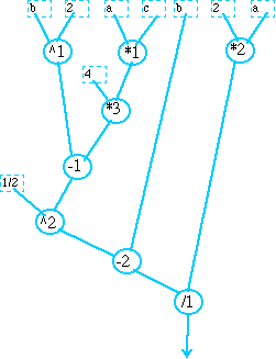
x= div(sub(pow(sub(pow(b,2),mul(mul(4,a),c)),1/2),b),mul(2,a))
The functional representation expressed in the above equation when diagrammed, gives insight into the parallel structure of the computations.
This is clear from the resulting computational graph shown in Figure 2-1. In this figure the input elements are the variables a , b ,c and the constants 2, 4, and 1/2. The function operations are *, ^ , - and / which are mul, pow, sub and div respectively. These operations are represented in the graph by nodes We attached an additional label to the operations to distinguish the instances of the same operations. As is evident from the graph, the longest chain of computations beginning with mul(a,c) will require six operations to complete the computation. The operation mul(2,a) only needs two operations. While this computation graph gives effective insight into the computation required by the algorithm, other refinements in the graphical representation can be added to give a complete description of the computational behavior of the algorithm and to include the temporal nature of the computations. The computation graph as presented, just shows the precedence relationships among the individual computations. When the computational graph is executed the temporal nature of the computations comes into play.
For our example let us assume that all the operations take a unit time to execute. We begin the development of the timeline of the execution by assuming at time = 0 that the variables and constants have been assigned values. Figure 2 - 2 is a timeline of the executions showing the maximum parallelization of the computations.
In this figure each operation is given a unit execution time. We have assumed that the data transfer as indicated by the arrows from the parallel computations is executed in zero time.
The computation graph expresses precedence among operations. In order to reuse the computation graph on successive sets of input variables we need a new form of graph. In order to formalize the expression of this successive computation mechanism we develop the DF graph. The values of the input and intermediate variables which are represented by an arc in the computation graph become the storage locations for these variables. The mechanism of storage of these variables is First In First Out or a FIFO queue. The quadratic root DF graph is set up by initially loading an input set of queues with values of the variables a, b, and c. The nodes of the DF graph now represent the computations that are performed upon the set of data items obtained from the input arc or input queues associated with this node and the output data items are placed on the output queue. In order to allow the temporal nature of the computation to be expressed in the DF graph the concept of threshold is introduced. Each node has the capability of checking all its input queues and when there is sufficient data on all the queues that exceed the threshold, the node executes and produces the output. After the node executes or fires the input data is removed from the input queues. With this firing mechanism implied in the graph, the DF graph representation now contains, in addition to the data values, control information that controls the execution of the graph. The actual sequence of computation represented by the DF graph is now not a simple linear execution of the nodes as it was with the computation graph.
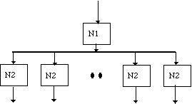
A simple example illustrates the basic nature of the DF graph as differentiated from the computation graph. This DF graph consists of a two nodes shown in Figure 2-3. The first node is a node has a input threshold of 1 and produces 10 pieces of data. The next node in the Data Flow graph has a threshold of 1. When the first node fires 10 data items are placed on the interconnecting arc or data queue that this arc represents. The second node will now have to fire 10 time to remove the ten data items from the intermediate queue. The actual computation graph would now show the first node and then 10 second nodes as Figure 2-4.
The next issue addressed is when the first node fires, the 10 data items it produces are now available. These items can be processed in cascade creating 10 firings (see Figure 2-4) of the second node or the 10 data items can be placed in 10 queues and the second node can be replicated 10 time so that we may process all the data in parallel. We can draw a new DF graph to represent the required parallel computations as shown in Figure 2-5. The individual second node computation nodes must then be mapped to individual processors in order to enable the parallel computation. The purpose of this parallelization and mapping of the computations is to reduce the computational latency of the algorithm execution. In the execution order of the first DF representation of Figure 2-3 it takes 11 execution times to produce the output from the 1 input data item. If the executions were performed in parallel as shown in figure 2-5 then the computational latency can be reduced to 2. This simple example shows that in order to be able to achieve parallelization the DF graph must be altered to express the parallelization.
This example illustrates the task of the graph designer. Even though the two DF implementations produce equal functional results, the two node Data Flow graph originally proposed must now be altered to produce an 11 node graph in which the first node produces 10 items and each output of the first node is followed by a single second node. This example illustrates that the design of a Data Flow graph is affected by the requirement of computational latency. When the problem requires parallelization in order to achieve this requirement, the design process or capture process of the algorithm to the DF graph must include the parallelization constructs or nodes. The next section discusses the alternative type of node specifically needed in the DF graph to implement parallel forms of the algorithm.
2.0 Introduction to Graphical Data Flow Description
Graphical representations of computations have been developed to provide an insight into sequence of computations. A complete process has been developed that begins with the translation of the requirements for a signal processing problem description into a Data Flow (DF) graph. This process allows the designer to rapidly progress from the signal processing algorithm to executable code that is automatically generated to run on the target COTS DSP processors. A supporting set of tools have also been developed to simulate and verify the design and to provide timing and memory sizing of the final executable code. These tools automatically autocode the DF graph and generate executable code that loads and runs on the target DSPs. While the tools automate most of the mechanical procedures involved, there are important design considerations in the design of the DF graph that affect the final executable code. This paper presents these considerations and discusses the design options in the DF graph design:
2.1 Computation Graphs
The graphical notation that is used to express a set of computations follows a functional description of these computations. We use c = func(a, b) to represent an arithmetic operation performed upon the elements a and b to obtain c. The elements may be single numbers, vectors or matrices. The elements may also be structures that are mixtures of numbers represented as integers and/or floating point numbers with different precision. It is also possible to have the elements represent characters.


2.2 Data Flow Description
While the computation graph expresses some of the aspects of the computation we extend the graphical description of the computation to encompass additional attributes of the computation. The graph that results is called a Data Flow (DF) graph.


![]()
![]()
![]()
![]()
Next: 3 Introduction to Data Flow Graph Design
Up: Appnotes Index
Previous:1 Executive Summary