Next: 4 Concept of State Up: Appnotes Index Previous:2 Introduction to Graphical Data Flow Description
![]()
![]()
![]()
![]()
Next: 4 Concept of State
Up: Appnotes Index
Previous:2 Introduction to Graphical Data Flow Description
In the introductory discussions of DF graphs, we have only introduced the processes of data distribution. When the data resides on the same processor that performs the computation, the data is not moved but a pointer to the data is transferred between the consecutive processing nodes. When the processing nodes are separated on multiple processors, the data is actually copied from one processors memory space to the other. The copying process actually takes a finite time to execute. The designer must be aware of this time but usually, in the early stages of the design, the data movement time is assumed to be negligible or easily accommodated by adding an additional processing time to each node's computation time. As the design progresses the actual transfer time is included in the simulation to verify that the system has met its latency specification. In the next section we introduce the set of specialized nodes that are used to copy and replicate the data so the DF graph can express the parallelism in the algorithm.
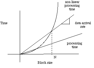
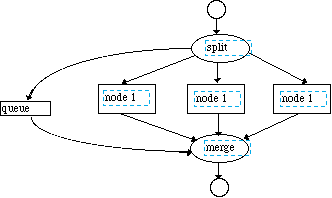
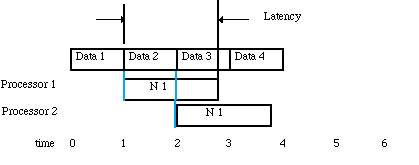
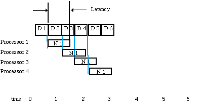
This block size can be found by equating the block arrival rate to the block processes time as shown in Figure 3-3. In the case where there is no solution for any block size or it is impractical to use the solution block size, then the processing must be parallelized as shown in Figure 3-4. The parallelization procedure begins by inserting a Splitter node which will send the first block of data to node1 and the second block to node2 etc. If the nodes are distributed to separate processors then the time line shown in Figure 3-5 results. For this method of parallelization the timeline shows that the latency that is greater than one block processing time. In this case, the latency can be decreased by using a smaller block size and using more processors and this is shown in Figure 3-6. This figure shows that we have cut the latency by a factor of two by increasing the number of processors by a factor of two. This is possible when the processing time is a linear function of the block size.
The other node that is shown in Figure 3-4 collects the data stream and is called the merge node. This node actually fires when a block of data arrives on one of its indicated input nodes. Strictly speaking, the merge node does not behave as an ordinary DF node. The rule for firing a DF node is that the node fires or computes an output when all the input queues are over threshold. In the case of a merge node, only one of the input nodes will be over threshold at a given time. In practice, the merge node uses an additional queue of control data generated by the split node that indicates which of the input queues should be examined by merge node for the queue over threshold signal. This additional queue is shown in the graph of Figure 3-4. This control node assures us that the merge node will reassemble the data blocks in the same order that they were split apart by the splitter node.
In the SAR example (see SAR Case Study) the split - merge pair was used to distribute the range processing data to each node. The graph also made use of the Family notation so the discussion of this graph will be deferred to Section 3.4.
processing is shown is executed between the split and merge nodes and a Family notation is used for the range processing nodes. The external feed-forward queues are shown that feeds the control queue from the split node (dfc_swth) to the merge node. The addition of the dfc_rep node in this path was used because of the configuration of the dfc_swth node that was used to implement the control feed-forward. Since the azimuth processing could not proceed until a full frame of range data was processed, the azimuth processing uses a Sep and Cat pair. This pair was used to implement the corner turning required by the SAR processing. The processed range data could only be distributed only after the queue following the merge node contained a complete frames worth of data. A Transpose node could have been used to perform the corner turning but in order to perform the azimuth processing in parallel, a Sep node would still have to follow the transpose node. Therefore the transpose operation was performed by the Sep node in addition to the parallelization of the data stream. Again the azimuth processing nodes are represented using family notation.
Because of the setup time for a single block of range processing was large for each individual block, the input blocks of data were grouped together and the range computation node was performed on a group of blocks at one time. The range processing node included a loop for each block of range data even though the inner processing was still performed on a range block by range block basis. Since all the computations were performed on one processor the successive range computations could be pipelined so that the setup time was only present for the first range block and the overall processing time reduced. The additional latency caused by the range computation being performed over several blocks at a time was acceptable. This latency is small compared to the amount inherent in the corner turning operation of the SAR computation. A full frame (range by azimuth block data size) latency exists as a minimum even in addition to the azimuth computation time.
This technique is illustrated by the ETC graph.(see the ETC4ALFS on COTS Processor Case Study for additional information regarding this application).
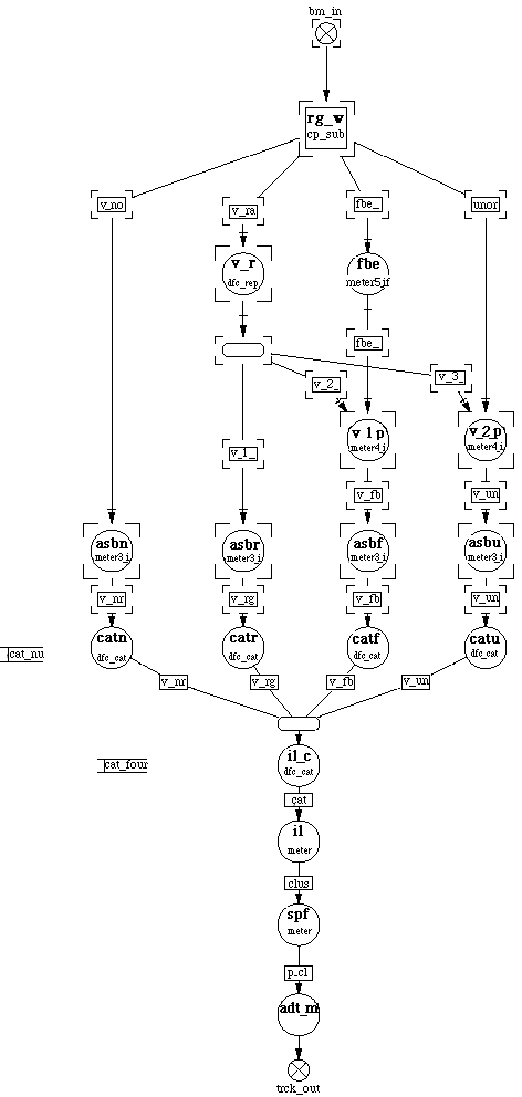
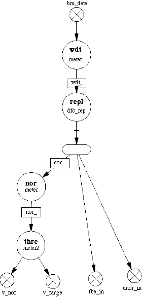
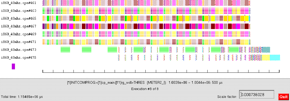
The family output data streams were then combined as shown using the CAT node. The Processing was then completed by as set of sequential nodes. This DF graph design was tested with sequential data streams and the integrity of the DF design established. By using a performance simulation tool and assigning representative processing time for the processing nodes (meter nodes) a execution time line was developed. This is shown inn figure 3-12.
The Processing was divided onto 8 processors. In this initial design the node processing times were approximated by a simple linear time formula as a function of the block size N. Processing time for a node is tnode = a + b N formula where a and b are processing times and N is the number of data item processed per node firing.
3.0 Introduction to Data Flow Graph Design
In this section, we will show how a set of algorithms that make up a signal processing algorithm can be converted to
3.1 Parallel Constructs
A DF graph is an ideal tool for representation of course grain parallel data processing. Coarse grain processing is best illustrated by example. In the example discussed in Section 2.0, the graph represented operations upon single data items such as a, b, and c and produced one result, x, the root. In general, the setup time for the functional calls needed to implement the computations represented by the nodes of the graph, will exceed the time it takes to execute the single functional operation performed by the node. Thus using a series of nodes to perform a sequence of operations will increase the overall execution time of the graph. In order to spread the setup time for a single node computation over many computations the graph is made coarse grained or each node is made to operate on a group of data each time it is fired. An example of this coarse grained operation would be the operation of an FFT node. The FFT function would operate on a data set or a vector and produce a vector of data for each FFT operation. Very often, even single operations as those implied by the computation graph in Section 2.0, can be converted to vector operations. Each of the of a items of a, b and c can be grouped into a queue of a, b and c and a single computation node can be made to include a loop to operate on each of the input items sequentially. From a graph point of view, the new graph is now coarse grained. Once the processing is put on a coarse grain basis each of the node operations can now be distributed. By assigning different nodes to different processors the processing can be performed on multiple processors simultaneously thus parallelizing the signal processing problem. The graphical notation used to express this data separation is the node constructs of SPLIT or SEP(aration) and the rejoining primitives of MERGE or CAT (concatenation). The use of each of these techniques will be discussed and illustrated by examples in the following sections. Other data organization elements such as MUX, and DEMUX will also be discussed.
3.2 Splits and Merges-Sequential Splitting
Usually data arrives at the input queue in a steady rate and this data must be processed sequentially by a computation node as shown in Figure 3-1 There are two methods of processing blocks of data so that the processing can keep up with the input data rate. The first method assumes that the node can complete the processing of the first block before the second block shows up. In this case, as shown in Figure 3-2, the latency or the time it takes to produce the results of processing the first block of data is less than it takes to process a block of data. If there exists a nonlinear trade off curve between block size and processing time, a block size can be determined that allows the computation rate to keep up with the data arrival rate.


3.3 Sep(aration) and Cats(concatenation)
When the input rate is large compared to the processing rate we can assume that the input queue is filled instantaneously. In this situation, the split and merge can be replaced by the Separate and Concatenate node. These operations are functionally similar to the split and merge nodes but the Sep node requires that the N blocks are present in the input queue before the node fires. N is the number of streams that the input block will be separated by the Sep processing node. Similarly the Cat node takes the N input nodes and following the DF rules fires when all the N input queues to this node are present. This combination of nodes is shown in Figure 3-7. In the figure the sep_a node uses the dfc_sep primitive and the mux_a node uses the dfc_cat primitive. The usage of the Sep - Cat pair is similar to the Split - merge pair but the Sep- Cat obeys the Data Flow rules and does not require the additional control queue that insures that the proper firing sequence is maintained.
There is another primitive node that can be used to separate data streams. This node is called DEMUX. The multiplex operation separates an N block queue into N streams but the data is not taken in contiguous blocks from the input data stream as in the Sep node. There is a stride applied to the selection of the data items from the input steam. The resultant output block now contains a group of data in which each consecutive item comes from the input stream and was separated by the stride from the next data item in the input stream. The corresponding concatenate operation is called MUX and reassembles the data stream.

3.4 Family Notation
In DF graphs we introduce an important notational construct that supports parallelization and it is family construction. By the use of this construct, a group of nodes and or storage queues may be vectorized. The individual entities are directly addresses by an index. This convenient notational technique allows the graphs to be simply constructed. For example if a Sep and Cat operation are used, the intervening node can be put into a family index notation. The family notation is shown conceptually in Figure 3-8. In this case the output of the Sep node is put into inq family of queues indexed by i = 1..n. In this example we feed [i]inq to [i] node and feed the output queues [1..n]outq to the CAT node. The Cat node is set to take a family of queues. The Family notation can be used on a graph that has routing complexity that is greater than the simple one to one routing shown in the example given. To accommodate this complexity a routing box can be inserted after inq to route the output of queue [i]inq to any node in accordance with a routing formula on the index i or expressed using a routing graph that can be explicitly drawn.

3.4.1 Examples of Family Notation.
In the SAR example the split - merge pair was used to distribute the range processing data to each node. In this manner each set of range cells could be processed in parallel. The graph was developed with the split node because the range processing time was greater than the time it took for one range block data to arrival.
Figure 3-9 shows the overall graph for the SAR processing. In this case the range

3.5 Data Flow Design Verification
After the DF graph has been constructed using the appropriate parallel constructs, a simulation should be set up to verify that the data stream is operating as desired. A graph can be set up using:
The initial input data streams can be made to be a simple sequence of numbers. As the data is passed through the node of the initial Data Flow design the integrity of the data stream can be verified.
![]()
![]()
![]()
![]()
Next: 4 Concept of State
Up: Appnotes Index
Previous:2 Introduction to Graphical Data Flow Description