Next: 4 Integrated Toolset Example for COTS Architecture Up: Appnotes Index Previous:2 Introduction
![]()
![]()
![]()
![]()
Next: 4 Integrated Toolset Example for COTS Architecture
Up: Appnotes Index
Previous:2 Introduction
In the systems process, processing requirements are modeled in an architecture-independent manner. Processing flows are developed for each operational mode and performance timelines are allocated based on system requirements. Because this level of design abstraction is totally architecture-independent, HW/SW codesign is not an issue.
In the architecture process, the processing flows are translated to data flow graphs and control flow description for subsequent processes. The data flow graph(s) becomes the functional baseline for the required signal processing. The processing described by the nodes in the data flow graph are allocated to either hardware or software as part of the definition of candidate architectures. This becomes the transition to architecture dependence.
The HW/SW allocation is analyzed via modeling of the software performance on a candidate hardware architecture through the use of both software models and VHDL token-based hardware performance models. For selected architectures requiring:
Reuse library support is an important part of the overall process. The methodology supports the generation of both hardware and software models. Software models are validated using appropriate test data, and VHDL hardware models are validated using existing, validated, software models. When a hardware model also requires new software - such as a new interface chip requiring a new driver - the hardware and software models are jointly iterated and modified throughout the design process.
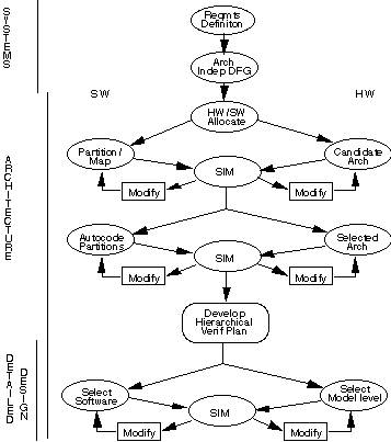
Simulation is an integral part of HW/SW codesign. Figure 3 - 2 shows a top-level view of the simulation philosophy in the RASSP methodology. During the systems process, functional simulation is performed to establish a functional baseline for the signal processing application. This functional baseline is architecture-independent and may be generated using a variety of tools for algorithm development and simulation including MATLAB, PGM Tools or GEDAE™. System designers may make an initial estimate of hardware / software allocation and obtain early cost estimates from tools like PRICE based on these allocations.
During the architecture design process, various simulations are performed at differing levels of detail as the design progresses. Early in the process, performance simulations are executed using high-level models of both hardware and software from the reuse library. Software is modeled as execution time equations for software primitives executing on various processors in the architecture. The architecture is described using token-based performance models for both the processing elements and communication elements. This level of simulation facilitates the rapid analysis of a broad range of architectural candidates composed of various combinations of COTS processors, custom processors, and special-purpose ASICs. In addition, many approaches to partitioning and mapping the software for execution on the architecture can be evaluated.
As the architecture process progresses, each of the software graph partitions is automatically translated into a software module for execution on a specific processor in the architecture. Functional simulation is used to verify that the generated code is consistent with the functional baseline. Performance simulation provides the next level of assurance that all throughput requirements are met by using lower level models, including the operating system, scheduling, and support software characteristics. Finally, hierarchical architecture verification of the architecture is established using selective performance and functional simulation at the ISA and/or Register Transfer Level (RTL) level. The goal is to ensure that all architectural interfaces are verified.
In the detailed design process, selective performance and behavioral simulation are performed again. At this point, however, the design has progressed to the point where simulation at the RTL and logic levels is most appropriate. Verification of the designs at this level is necessary prior to release to manufacturing. It is important to note that pieces of the design may be in different stages of the overall process based on the risk analysis performed in each development cycle. For example, if it is obvious to the designers during systems definition that they will need a new custom hardware processor to meet the requirements, they may accelerate the design of the custom processor while the overall signal processor design is still in the architecture process.
In order to perform architecture tradeoffs, a candidate architecture must be postulated. This can be accomplished graphically as will be shown in subsequent paragraphs. Underlying each of the elements in the hardware architecture is a token-based performance model. As part of the effort required to perform the architecture tradeoffs, any models or variations of existing models which do not exist but are needed to represent candidate architectures must be created. Refer to the Token-Based Performance Modeling application note for the development of these models.
The required processing time for each of the functions in the processing flow must be obtained. Initialy, these times may be estimated and can be updated as implementation details become better defined. After having both a processing flow and a candidate archtecture, various mappings of the required processing to the candidate architecture can be postulated. In each case, the expected performance is simulated and either the architecture or the mapping may be modified to optimize performance. Simulations may be performed using state of the art tools for constructing the simulations and standard VHDL simulators.
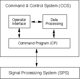
A typical large scale conceptual architecture is shown in Figure 3 - 4. It consists of a Signal Processing System (SPS) communicating with a Command and Control System (CCS). The Signal Processing System is that portion of the overall application that performs the high bandwidth "number crunching", is naturally represented by a data-flow model of computation, and typically executes on Digital Signal Processors (DSPs). Intimately related to the SPS, but frequently conceptualized as part of the Command and Control System is the Command Program (CP).
The Command Program serves as an interface between the SPS and the rest of the CCS by translating system derived or user inputs into sets of commands that are understood by the SPS and by forwarding SPS results. It is significantly more than a simple data reformating program. The CCS system views the SPS as a collection of domain specific abstractions that are frequently refered to as modes and submodes. For example, in an airborne radar, the CCS system may view the SPS as performing "the weather mode" or "the track submode of the Airborne Target Search and Track Mode". However, the notions of mode or submode are foreign to the SPS. The fundamental concept in the SPS system is that of a graph, while a mode may correspond to a collection of concurrently executing graphs. The SPS is modeled using the Data-Flow paradigm, while the Command Program is often represented by a Finite State Machine. Thus the command program must transform the CCS notions of mode and submode into the SPS notions of graphs and dataflow.
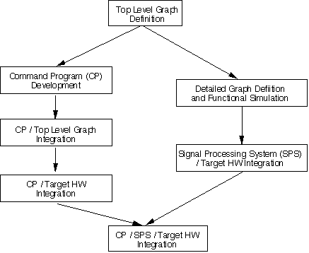
Another representation of the command program and signal processing software development process is shown in Figure 3 - 5. The first step is to capture the set of graphs to be controlled by the command program. This depends only on knowing the set of modes and submodes, which may already be defined in the procurement specification, and the top level assignment of signal processing algorithms to a set of signal processing graphs. Command Program development is not dependent on the detailed implementation of the signal processing graphs whose implementation is shown on the right hand side of Figure 3 - 5.
After the top level graphs are captured, command program development proceeds. Following CP development, the CP is integrated with the top level graph. The Top Level graph at this stage only needs to perform data flow adequate to exercise the command program. Since graphs can easily be retargeted in GEDAE™ this integration can be performed on the CP development host. The next step is to verify that the actual command program executes as expected with the target hardware and in cooperation with the rest of the command and control system. This can also be performed independently from the detailed signal processing. The approach is to again use the top level graph but to retarget its execution to the final target hardware; this is easy to do in the GEDAE™ development environment. Concurrent with the development of the Command Program and its integration with the top level graphs, the DSP application graphs are being completed and tested on the target hardware. When the signal processing graphs are completed and tested, the final system integration uniting the command program and the final signal processing graphs may occur.
After the top level graphs are captured, command program development proceeds using Verilog's ObjectGEODE tool. The model is simulated with the interface to the actual data flow graphs implemented as a set of smart stubs. A smart stub is a software program which simulates simple responses from the signal processing system. Command program functionality can thus be verified independent from the implementation of the signal processing. Concurrent with the command program development is the detailed definition of the application graphs in GEDAE™. The top level graphs are detailed and simulated using GEDAE™ to establish correct funtionality.
The assumption in the discussion that follows is that the hardware and software models required to construct an architecture and/or signal processing graph exist in a reusable library. Although this assumption is made for the purposes of discussion, many of the graph primitives used in the application were generated specifically for this application. In general, new primitives will often be required and consequently tools must support easy primitive generation and insertion into the system. In addition to the three tools shown in Figure 3 - 6, ATL has developed an Application Specific Interface Builder (AIB) which is also discussed. Its purpose is to provide a more natural interface between the signal and control processing. The example used in the following discussion is the SAIP (Semi-Automated IMINT Processor) application which was the 4th RASSP Benchmark.
Overview - GEDAE™ is a highly interactive graphical programming and autocoding environment which facilitates application development, debugging, and optimization on workstations or embedded systems. It's graphical editor supports building data flow graphs which are very readable. Explicit inputs and outputs are identified and user notes can be inserted directly on the graph canvas. The same user interface which supports the graphical editor is used for controlling all activity within GEDAE™. It is not necessary to switch tools or become familiar with a different user interface when moving from algorithm development to embedded code generation which minimizes the learning curve and reduces tool training. The interface has been aclaimed as highly intuitive by observers at conferences and the visualization is unmatched for analizing system solutions. The overall philosophy employed in the development of GEDAE™ is "never take intelligent decisions out of the hands of the designer - but rather provide the tools and functionality needed to improve productivity and decision making, automating as much of the drudgery as possible". Capability is provided for the designer to readily partition graphs and map the partitions to multiple workstations or multiple processors in an embedded system. Autocoding generates appropriate schedules and code for each processing element which is efficient in terms of execution time and memory usage.
A GEDAE™ Run-Time Kernel provides all of the interprocessor communication required by the particular software mapping. Although the designer has flexibility in selecting the type of communication used (e.g. socket, DMA, or shared memory), implementation of the communication is automatic. Therefore, the application developer never needs to write any interprocessor communication software. This may in fact be the largest benefit of graph based programming for multiprocessors since our experience indicates this area to be responsible for most multiprocessor system debugging problems.
Algorithm Capture - Algorithms are captured in GEDAE™ by placing processing functions extracted from a library on a canvas and interconnecting them using the extensive facilities of the graphical editor. Using a top down design approach, the basic building blocks and data passing requirements can be put on the canvas. In this way, the application designer can build, test, and analyze algorithms with point and click simplicity. Designers can select from functions contained in the extensible library. Library functions are provided for most of the commonly used signal processing functions. Understanding that a function library will never be complete, templates are provided for creating new functions. In addition to providing all of the typical data types, GEDAE™ has the important capability to define new arbitrary data types(e.g. complex C structures) for use with custom primitives. This ability is of great importance to users who want to capture heritage software which is generated in modules whose I/O is maintained as complex data structures.
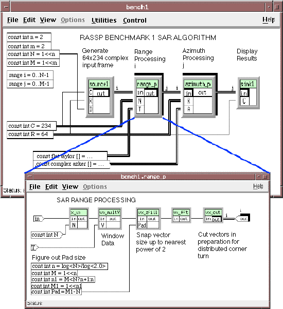
Hierarchy is supported in a flow graph which simplifies complex application understanding. A typical hierarchical graph is shown in Figure 3 - 7 with the hierarchical function titled "range_p" expanded. The application is Synthetic Aperture Radar(SAR) image generation which was used as a benchmark on the RASSP program. All functions in the top level graph are hierarchical and can be expanded by double clicking on the box title bar. Unlimited nested hierarchy is supported.
GEDAE™ supports extensive and efficient parallel processing. Parallelism is succinctly represented in the SAR graph. The bold shadow surrounding some of the graph nodes as well as some of the node inputs and outputs indicates a 'family' of functions and the double lines between nodes indicate a family of interconnects. The indices above any family function (e.g. "i" above the range_p box) indicates that there are "i" of these functions. The output of the source1 box is a family of "i" outputs for processing by the "i" range_p functions.
The familly of outputs is represented by the shadow around the source1 "out" label and the label "i" on the arc. In addition the output of each range processing family member is also a family which indicates that each section of data processed by one of the range processing functions is output as a family of outputs. When embedding this application, the individual family members are mapped to different processors for concurrent processing. Of particular note is that the alternating indices between the output of range processing and the input to azimuth processing specifies a distributed corner turn since the "j-th" output from the "i-th" range processor is routed to the "i-th" input of the "j-th" azimuth processor.
When the interconnection of the links between family members becomes complex, special routing boxes can be inserted to define the connections. These routing boxes are merely a graphical representation aid and do not consume processing resources.
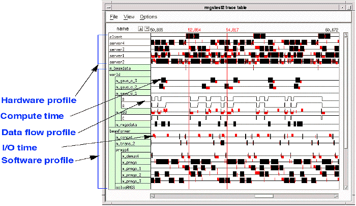
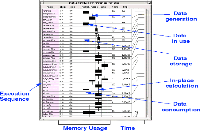
Simulation / Validation - Execution of GEDAE™ graphs is controlled through the same interface used to construct the graph. Users can modify parameters in the graph on the fly and observe t2he impact of those changes. The ease of making modifications to a graph and its operating parameters increases productivity by making it easy for designers to fine tune applications quickly. Execution results are presented to the designer in the form of detailed timelines and execution schedules along with memory maps to support the designers analysis of system solutions. An annotated example of a trace table is shown in Figure 3 - 8. It contains both a hardware execution profile and a software execution profile. Computation time, data flow activity(buffers filling and emptying), and communication activity are all detailed in the trace table.
Embedded Code Generation - GEDAE™ provides an efficient autocoding capability driven by partitioning and mapping defined by the user. Because GEDAE™ handles all interprocessor communication, the designer never has to write any communication software. GEDAE™ launches the compilation, linking, loading and execution of the application on the embedded hardware. An embedded run-time kernel on each processor supports execution. GEDAE™ generates the execution schedule for each processor and provides the user the ability to divide schedules into sub-schedules which may all operate at different firing granularity to optimize performance. Execution schedules and memory maps are presented for analysis as shown in Figure 3 - 9.
Optimization - GEDAE™ supports the optimization of partitioning and mapping, memory usage, communication mechanism selection, schedule firing granularity, queue capacities, and scheduling parameters. GEDAE™ provides the ability to interactively manipulate these items which greatly improves the designers ability to optimize processing after retargeting an application to a new architecture.
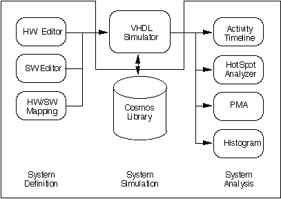
Using Cosmos, the user builds a model of a system. A model consists of hardware elements connected together into the schematic of the system, software tasks that model the software components of the system, and a mapping that defines which software tasks run on which processors in the system. After a model is built, it is simulated using a commercial VHDL simulator. The simulation results are then imported back into Cosmos to be analyzed. Cosmos includes a complete set of analysis tools that allow the user to look at the behavior of the system in detail, and identify potential problems such as network bottlenecks, insufficient processing power etc. Cosmos provides a complete set of versioning and data storage features so that different versions of a system model can be saved and compared to each other for choosing the best version.
Cosmos Usage - Cosmos models systems using a VHDL based library of elements such as processors, networking elements etc. The models are un-interpreted, token-based models, in which actual data is not simulated, but only the interaction of elements based on the size and other characteristics of the data is simulated. This allows a very large increase in simulation times (by a factor of as much as 1000 over full-functional simulation), and also allows large systems (consisting of tens or hundreds of processors) to be simulated easily.
The Cosmos user builds a model of a system using the library elements for the hardware description. This is done using a built-in schematic editor. The hardware elements in the library include various commercial processors, networking elements such as VME, Mercury Raceway and Myrinet, and other data processing elements such as memories, disks, and data generators and data sinks. The various elements are instantiated into a system model and each instance can be customized by changing the values of parameters such as latency, throughout and other element-specific parameters. The elements are connected together in the schematic editor to define the hardware architecture of the model.
The software description is built using flow-charts, each of which represents a task running on one or more of the processors in the system. Each processor element in the library supports a real-time multi-tasking OS model, which can be customized to simulate the performance characteristics of different operating systems such as MCOS and VxWorks etc. The OS model also supports built-in inter-task communication mechanisms that allow different tasks to communicate with each other. A task in the software description of the model can simulate execution of instructions by using built-in mechanisms of the processor model. This allows the performance of the task to be modeled. The task is independent of the processor it runs on, so it is possible to model the performance of the same task(s) on different processors to understand the impact of changing processor architectures.
The tasks defined in the software model are mapped to the various processors instantiated in the hardware model using a mapping editor. This allows the user to easily change the mapping of software to hardware in the system model, without changing the hardware or software models.
Once the system hardware, software and mapping are defined, Cosmos generates a VHDL model of the system. This model uses a Cosmos supplied, VHDL based library as a basis for simulation of the system. The simulation is performed using a commercial VHDL simulator (Cosmos supports all the leading VHDL simulators). The simulation results are imported back into Cosmos to be analyzed, using the Cosmos analysis tools.
The simulation results can be analyzed using various tools that allow the user to examine the simulation as a whole, or examine the activity in the system at a given instant of time. The simulation can be played and/or stepped through forward or backward to examine events in sequence. The analysis tools include the Activity TimeLine, the HotSpot Analyzer, the Performance Metric Analyzer, and the Histogram Tool. The Activity TimeLine displays the entire simulation as a plot of time vs. activity of each individual hardware instance and software task. The TimeLine display shows overall activity of the system, and any specific activity can be examined in detail to indicate what each element and task was doing at any given time. The HotSpot Analyzer shows the utilization of the hardware elements in the system at any given instant of time. As the simulation is played back and forth, the HotSpot shows element utilization on a color-temperature scale. This makes it easy to detect over-utilized or under-utilized elements in the system. The Performance Metric Analyzer (PMA) shows the instantaneous values of various performance metrics such as utilization, latency and throughput for any set of elements in the system. The Histogram Tool allows the user to plot these same metrics for the simulation as a whole, giving a picture of the performance of an element over the entire simulation.
Figure 3 - 10 shows the relationship of the various elements of Cosmos.
ObjectGEODE supports a coherent integration of complementary approaches based on standards. These standards are:
OMT/UML Class, Instance Diagrams and StateCharts are used to perform system requirements analysis. SDL includes Architecture Diagrams for system structure, Interconnection Diagrams for system communication and Extended Finite State Machine Diagrams for system behavior. MSC includes Message Sequence Charts for Use or Test case definition and Scenario Diagrams grouping Sequence Charts for function description. Data can be described with ISO's ASN.1. All these diagrams are closely interrelated thus removing any possible discontinuity right through to the final implementation stage.
The OO approach implemented in ObjectGEODE, supports project members on a long-term basis and takes reuse into account at all levels.
ObjectGEODE features - ObjectGEODE provides the following features.
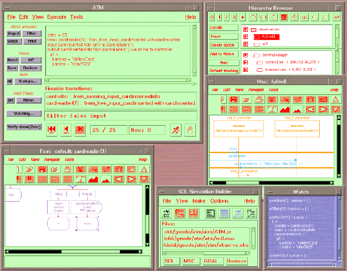
Figure 3 - 11 shows a typical screen from an ObjectGEODE simulation session.
Host and Target Systems Supported - The ObjectGEODE toolset runs on SUN, HP, IBM RS/6000, DEC Alpha workstations and on Windows NT. Most popular target systems such as VRTXsa, pSOS+, VxWorks,or UNIX are supported as well as TCP/IP for distributed communications.
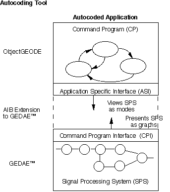
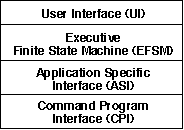
The overall command program is a layered architecture as shown in Figure 3 - 13. The bottom two layers address the data flow graph perspective while the top two layers address the control perspective. The bottom most layer is the Command Program Interface (CPI) layer and consists of the generic set of graph control functions provided by GEDAE™. This layer can be viewed as Commercial of the Shelf (COTS) software from the perspective of the command program. The next layer is the Application Specific Interface (ASI) layer. It is generated by the Application Interface Builder (AIB) and provides a high level set of functions used to instantiate, control, and configure a top level graph(s). The next layer up is the Executive Finite State Machine layer that reflects the state of the signal processing application. This layer may reflect a wide range of complexity and may be generated by hand or may require the utilization of a graphical tool such as ObjectGEODE. The User Interface layer may represent a simple interface for testing or may represent a complete interface for the application.
3.0 RASSP Hardware / Software Codesign Process
3.1 Definition and Benefits
HW/SW Codesign refers to the simultaneous consideration of hardware and software in the design of a system, rather than the more common approach of specifying the hardware and constraining the software to fit. The RASSP program therefore defines HW/SW codesign as the co-development and co-verification of hardware and software through the use of simulation and/or emulation. This codesign begins with Functional Design and ends with Detailed Design, as shown in Figure 1- 1, where Detailed Design includes software generation but not hardware fabrication. The principal benefits of HW/SW codesign are that it:
3.2 Implementation of Hardware / Software Codesign in RASSP
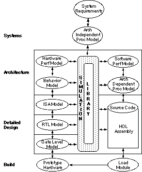
The RASSP design process is based on true hardware/software codesign and is no longer partitioned by hardware and software disciplines but rather by the levels of abstraction represented in the system, architecture, and detailed design processes. Figure 3 - 1 depicts the RASSP methodology as a library-based process that transitions from architecture independence to architecture dependence after the systems process.
a) new computational elements,
hierarchical verification is performed using finer grain modeling at the Instruction Set Architecture (ISA) level and below. During the detailed design process, actual software code is verified to the maximum extent possible.
b) interfaces, or
c) communication mechanisms
3.3 HW / SW Codesign Versus Application and Architecture
Both the application and the evolving architecture for the signal processor influence the way in which HW/SW codesign is applied within the methodology. Table 3 - 1 contains examples of various mixes between COTS and custom solutions for the signal processor. Although the table addresses only hardware, the software may, in a sense, also be custom or COTS. Depending upon the nature of the evolving solution, one or more portions of the design may be defined or implemented concurrently.
3.3.1 All COTS Solution
An all-COTS solution means that in addition to the architecture being all COTS, as shown in line 1, Table 3 - 1, the signal processing data flow graphs can be constructed from existing primitives in the reuse library. There will likely be control software that must be developed, but all of the signal processing can be developed by graphically constructing the data flow graphs . from existing library elements. These data flow graphs will be translated via autocode generation for execution on the target processors under control of the run-time system, which is built with an open Application Programming Interface (API) to standard operating system micro-kernels. When executed on the target hardware, optimized versions of the primitives are utilized. In this type of solution, the HW/SW codesign process is completed when a satisfactory result is obtained from the virtual prototype, which includes both function and timing. This virtual prototype is a VHDL simulation that models the architecture, the run-time system, the operating system characteristics and the autocoded software. It also uses detailed timing data for software performance estimates for the target processors generated during the autocode process.
PE Comm Element PE Interface Comm Network Board Comments 1. COTS CUST CUST CUST CUST Architecture built from available board Primitives and OS services are available from libraries 2. COTS CUST CUST CUST CUST Applicaiton requires custom topoliogy and new board design 3. COTS CUST CUST CUST CUST PE needs to be interfaced to new interconnect fabric, new board design requirements 4. COTS CUST CUST CUST CUST New communication elements 5. CUST CUST CUST CUST CUST Application requires new application specific PE 6. CUST CUST CUST CUST CUST Application requires full custom solution 3.3.2 New primitives Required
Primitives are the bulding blocks from which the data flow graphs are created. A primitive is the smallest element of software which can be allocated to a processor. Although the intent is to provide a wide range of primitives suitable for many applications, there will always be the need for the user to develop and add new primitives to the reuse library. New primitives may be required either because new processing algorithms have been developed or because specialized optimization is required to meet throughput requirements. When new primitives are required, the HW/SW codesign represented by the detailed design portion of Figure 4 may be initiated as soon as the need for the primitives is recognized. Thus the detailed design of a new primitive is performed concurrently with the continuation of the architecture definition process. Initially the architecture definition process may proceed using estimated execution times for the primitives to be developed. The HW/SW codesign of the primitive proceeds by using either existing hardware, if available, or an appropriate level model - such as the ISA model - to both verify functionality and optimize execution times. As the maturity of the primitive implementation progresses, the execution times can be back-annotated to update the performance simulations used in the architecture development process.
3.3.3 Custom Hardware Required
As indicated in Table 3 - 1, there are a variety of reasons why designers may need custom hardware to support the overall architecture being developed. Perhaps they have not interfaced the selected digital signal processor to the desired communication network and require a new processor interface. This may also require that the underlying operating system services, such as communication drivers, be updated to support the new interface. Alternatively, designers may determine that a custom processor is required for a specific part of the application in order to meet the throughput requirements. The designers may initiate the HW/SW codesign represented by the Detailed Design portion of Figure 3 - 2 as soon as they recognize the need for custom hardware. Thus, they may concurrently perform the Detailed Design of the custom hardware and the interface software along with the continuation of the architecture definition process. In these cases, they develop models of the hardware at various levels of abstraction to support the process. They concurrently develop the software required to use the new interface hardware or custom processor and use it in conjunction with the hardware models to verify operation and performance. As designers develop detailed timing data, they use back annotation to update prior performance estimates.
3.4 Integrated RASSP Architecture Toolset
3.4.1 Implemented Process
An implementation of the RASSP architecture design process specifically for COTS architectures is shown in Figure 3 - 3. The signal processing and control requirements shown in the figure are outputs of the systems design process. In the figure, the architecture process is broken into five subprocesses:
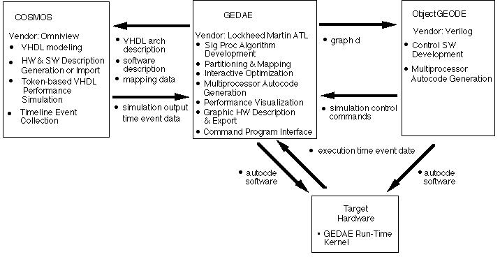
This overall process permits many of the above activities to be conducted concurrently. The integrated RASSP architecture toolset is based upon three tools, GEDAE™ from Lockheed Martin Advanced Technology Laboratories, Omniview Cosmos™ from Omniview Inc, and ObjectGEODE from Verilog SA.
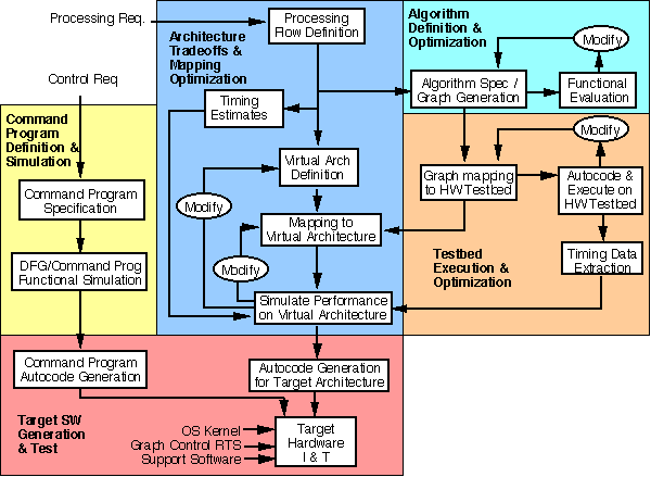
3.4.1.1 Architecture Tradeoffs & Mapping Optimization
The first step in the architecture tradeoffs is the generation of the required top level processing flows. It is not necessary to have a complete definition of the specific algorithms to be used, but it is necessary to have a definition and understanding of the data flow required. For early architecture tradeoff analysis, the algorithmic processing can be represented by time estimates (delays) for the computation. It is important however to have as accurate as possible representation of the data flow. The processing flow defines the way in which data must be moved from one algorithmic function to another. Depending on the mapping of the algorithm to the processors in the architecture, the passing of data from one processing function to another may or may not require moving data between physical processors or even between boards in the architecture. It is the data flow and the mapping of the required processing to the individual processors that will define the overall throughput achievable on a particular architecture.
3.4.1.2 Algorithm Definition & Optimization
Concurrent with the architecture tradeoffs, developers can be fleshing out the details of the algorithms. Each of the functions in the top level processing flows is replaced with the algorithmic details required by the application. Modern tools provide the ability to graphically construct the algorithm details, simulate the behavior of the algorithms to establish corrrect functionality and optimize the computation. As depicted in Figure 3 - 3, the algorithm definition and optimization is an iterative process which is simplified by graphical programming tools which provide detailed visualizaton capability.
3.4.1.3 Testbed Execution & Optimization
Once the algorithms have been defined, execution of the algorithms (or pieces of the algorithm) on a hardware testbed provides timing data which are more accurate than the original estimates used in the architecture tradeoffs. This new data is used to continually update the timing estimates and revalidate the performance of the selected architecture. The integrated RASSP archtecture toolset simplifies this process. This step can be especially usefull when the developers have access to a single board DSP testbed but the application requires perhaps tens of the boards. The testbed execution provides the accurate algorithm timing estimates and the performance simulation provides the confidence that the overall required data flow does not create crippling communication bottlenecks.
3.4.1.4 Command Program Definition & Simulation
Although the signal processing is the computational heart of an application, the overall control of the signal processing can often be very complex. The integrated RASSP architecture toolset provides assistance in this area as well. Depending on the complexity of the control that is required, it can be beneficial to consider the utilization of graphical programming tools and autocoding for the control as well as the signal processing. The command program definition and simulation indicated in Figure 5 may be accomplished graphically with modern tools that are specifically aimed at graphically specifying, simulating and autocoding software which is best described as a finite state machine. Joint simulation of both the control and signal processing ensures that proper functionality is maintained throughout control state changes. For details on the generation of control software see theAutocoding for DSP Control application note.
3.4.1.5 Target Software Generation and Test
When the candidate architecture is assembled, the autocoding capability of the signal processing and control processing development tools is used to generate the final software for the target architecture. The same visualization capability available during algorithm development and simulation is maintained through software debugging on the target hardware. The integrated RASSP architecture toolset provides the same user interface throughout the development process from concept to final software generation.
3.4.2 Integrated Toolset
As part of the RASSP development ATL has looked at a wide range of tools applicable to the HW/SW Codesign activity. These developments have resulted in the Integrated RASSP Archtecture Toolset. The intent of this toolset is to facilitate HW/SW Codesign through an integrated capability for specifying the signal processing application and its control, performing architecture tradeoffs using VHDL token-based performance models, defining the required functionality in the form of data flow graphs and control states, simulating the associated functionality of the data and control flow, and autocoding the final software (both signal processing and control) for the target hardware. These functions are performed using the GEDAE™, PMW (recently renamed Cosmos), and ObjectGEODE. Part of the RASSP effort has involved both enhancing and integrating these tools as shown in Figure 3 - 6.
3.4.2.1 GEDAE™ - An Algorithm Development/Autocoding Tool
This section briefly describes the GEDAE™ software, one of the tools in the HW/SW Codesign Toolset. Lockheed Martin ATL has been developing GEDAE™ for over a decade. GEDAE™ supports graphical programming and autocoding of applications for execution on workstations and embedded hardware. Under the RASSP program, GEDAE™ has been enhanced and integrated with the other tools in the HW/SW Codesign Toolset.
3.4.2.2 Omniview Cosmos™ - A Performance Modeling Tool
Cosmos from Omniview Design Inc. is a performance modeling environment that allows the user to quickly obtain data about a system's performance, such as latency and throughput. Both hardware and software components of a system can be modeled simultaneously. Cosmos is intended to be used as a high-level system design tool, where early design trade-offs in software/hardware partitioning and architecture are made. Currently, such trade-offs (such as the networking architecture to use, the number, type and speed of the processors to use etc.) are done on the basis of previous experience, spreadsheet based calculations etc. However, these calculations may not accurately capture the dynamics of the system, or may be insufficient to give the user an accurate prediction of the performance of a given system. Using a simulation based performance modeling environment such as Cosmos allows the user to obtain the performance characteristics of different system architectures early in the design cycle, thus allowing the selection of the best architecture amongst various alternatives before detailed design is begun. This potentially saves a lot of re-design and the associated costs.
3.4.2.3 ObjectGEODE - A Control Software Development and Autocoding Tool
ObjectGEODE from Verilog SA is a toolset dedicated to analysis, design, verification and validation through simulation, code generation and testing of real-time and distributed applications that are best represented by a finite state machine model of computation. Such applications are used in many fields such as telecommunications, aerospace, defense, process control or medical systems.
3.4.2.4. Application Interface Builder
As shown in Figure 3 - 12, the command program views the signal processing system as a collection of modes and submodes, while the signal processing system naturally presents itself as a collection of graphs. Consequently two interfaces are defined. The Command Program Interface (CPI) provides control services built around the signal processing graphical notions. The Application Specific Interface (ASI) provides a view of the signal processing as a collection of modes and submodes. The ASI is a more natural representation for system designers while the CPI is natural to the data flow graph designers. As Figure 3 - 12 illustrates, there is a gap between the two interfaces. An Application Interface Builder (AIB) has been developed by ATL under the RASSP program to generate the Application Specific Interface that fills this gap. The control software developer issues a mode change request via the ASI and the interface software constructed by the AIB will provide the detailed sequence of commands via the CPI to implement the request. The ASI instantiation consists of calls to the CPI based on the specific set of modes / submodes for the application, the set of graphs developed to perform the application, and the correlation between the two sets. The capability of the AIB will be commercialized as part of the GEDAE™ product.
![]()
![]()
![]()
![]()
Next: 4 Integrated Toolset Example for COTS Architecture
Up: Appnotes Index
Previous:2 Introduction